#Project #3: YouTube Attention and Review
#Group #7
#Jaydip Patel, Vincent Chang, Nicole Haberer, Ivy Wang, & Griffin Parr
Introduction
There are 98 files, both in revenue and video folder. There is also an additional file containing video metadata. Youtube account holder did a small research experiment, he created 98 videos and 50% of them contained ads and 50% were not. Then one certain day he switched the ad containing videos to non-ad containing videos and visa-versa. His aim to check, whether this action triggered high views in any section of videos or does the earning factor impacted?
This is an exercise in merging disparate data sources into a useful data set, and using the merged data set to perform some useful analysis.
PartOne >>>>>
Read in the revenue and the video data into separate objects (e.g., revs and vids), and then merge the revenue and video data into a common data frame that day x video observations on revenues and video characteristics for all of the videos (98 in total) and all of the days in the sample (from September 1, 2011 to March 20, 2012).
By the end of “Part 1,” you should have a fully assembled data set with the following characteristics:
• Each observation is at the date-video level.
• There should be fields for “daily_earnings” (“Total estimated earnings” renamed), “views”,
“average_watch_time” (“Average view duration” renamed), “video_id” (this should match the format of the “video.id” field from “adinstream.csv,” which we went over in class on Oct 8/9), and “DATE” (the date field, formatted as a “Date” object; see help(as.Date()), or Google information on Dates in R).
• Please also create variables within this data frame for “earnings_per_view” (daily earnings / views).
• You should also merge onto this dataset the “instream.csv” data set, which contains information about the experiment I ran regarding pre-roll ads placed on these videos. We discussed this in class (Experimenting
As a summary, produce both tabular and graphical summary information on daily_earnings, views, average_watch_time. Specifically, it would be useful to report the mean, standard deviation, and median of each of these variables. Also, produce a boxplot for each variable to summarize the distribution of values these variables takes on.
#author:  Team 7
#name:    #Jaydip Patel, Vincent Chang, Nicole Haberer, Ivy Wang, & Griffin Parr
#purpose: YouTube Attention and Review
#date:    2018.11.17
#version: R version 3.5.1

##global adjustments starts 01
rm(list=ls())
#seed for replication
set.seed(100)
oldwarnval <- getOption("warn") #preserve old value
options(warn = -1) #warnings are silent now
##global adjustments ends 01

revenues_fp <- "~/Downloads/Tony/Project 3/YouTube2013Attention/Revenues"
revenues_filename <- "/Users/Priyanka/Downloads/Tony/Project 3/YouTube2013Attention/Revenues/Revenue"
videos_fp <- "~/Downloads/Tony/Project 3/YouTube2013Attention/Videos"
videos_filename <- "/Users/Priyanka/Downloads/Tony/Project 3/YouTube2013Attention/Videos/Video"
adinstream = "/Users/Priyanka/Downloads/Tony/Project 3/adinstream.csv"

# function to read and merge data
folderdata = function(paths){
  dat = NULL
  for(i in 1:length(paths)){
    this = read.csv(paths[i], header=TRUE, stringsAsFactors = FALSE)
    this = cbind(this, paths[i]) #Read in the videoID
    dat = rbind(dat, this)
  }
  return(dat)
}
Read in folder
#Read in youtube folder
base = revenues_fp
yt_paths = list.files(base, full.names=TRUE)
revs = folderdata(yt_paths)
names(revs) <- c("Date", "Total.earn", "AFV.earn", "YT.earn", "Transactions", "VideoID")

revs[,6] <- gsub(revenues_filename, "", revs[,6])
revs[,6] <- gsub(".csv", "", revs[,6])

#Read in video folder
base = videos_fp
v_paths = list.files(base, full.names=TRUE)
vids = folderdata(v_paths)
names(vids) <- c("Date", "Views", "Est.min.watched", "Avg.view.duration", "Unq.cookies", "VideoID")

vids[,6] <- gsub(videos_filename, "", vids[,6])
vids[,6] <- gsub(".csv", "", vids[,6])
Merge files
#Merge vids & revs by Date
for(i in 1:nrow(vids)){
  if(is.na(as.Date(vids[i,1], format="%b %d, %Y")) == FALSE){
    vids$Date[i] <- as.character(as.Date(vids$Date[i], format="%b %d, %Y"))
  }else{
    vids$Date[i] <- as.character(as.Date(vids$Date[i], format="%d-%b-%y"))
  }
}
for(i in 1:nrow(revs)){
  if(is.na(as.Date(revs[i,1], format="%b %d, %Y")) == FALSE){
    revs$Date[i] <- as.character(as.Date(revs$Date[i], format="%b %d, %Y"))
  }else{
    revs$Date[i] <- as.character(as.Date(revs$Date[i], format="%d-%b-%y"))
  }
}

rv <- merge(vids, revs, by=c("Date", "VideoID"))
Colum adjustments
#rename columns
colnames(rv)[colnames(rv)=="Total.earn"] <- "daily_earnings"
colnames(rv)[colnames(rv)=="Avg.view.duration"] <- "average_watch_time"

#remove dollar signs and make daily_earnings column numeric
rv$daily_earnings <- as.numeric(gsub("\\$","", rv$daily_earnings))

#create earnings per view column
rv$earnings_per_view <- rv$daily_earnings/rv$Views

#drop column names we do not need
drop <- c("AFV.earn","YT.earn","Transactions","Est.min.watched","Unq.cookies")
rv1 = rv[,!(names(rv) %in% drop)] #new rv
Merge metadata colums on "Ads and NoAds, visa-versa"
#merge data with adsinstream.csv (describes pre-roll ads)
#import new csv file
instream <- read.csv(adinstream)
colnames(instream)[colnames(instream)=="video.id"] <- "VideoID"

##Instream videoID is poorly name--- rename to match rv1
instream$VideoID <- toupper(instream$VideoID) #all convert to upper case
rv1$VideoID <- toupper(rv1$VideoID)
setdiff(unique(rv1$VideoID), unique(instream$VideoID)) #output: "REG1"   "REG2"   "WHATIS" "REG3"
## [1] "REG1" "REG2" "WHATIS" "REG3"
instream[which(instream$VideoID == "REGRESSION1"),]$VideoID <- "REG1"
instream[which(instream$VideoID == "REGRESSION2"),]$VideoID <- "REG2"
instream[which(instream$VideoID == "REGRESSION3"),]$VideoID <- "REG3"
instream[which(instream$VideoID == "WHATISINTRO"),]$VideoID <- "WHATIS"

#Merge instream and rv1
rv1$annoy_before <- NA
rv1$annoy_after <- NA
for(i in 1:nrow(rv1)){
  if(is.na(match(rv1$VideoID[i], instream$VideoID)) == FALSE){
    n <- match(rv1$VideoID[i], instream$VideoID)
    rv1[i,c(7,8)] <- instream[n, c(3,4)]
  }
}
View the data and summary plots
#Data Summary & Analysis for Daily Earnings:
summary(rv1$daily_earnings)
##    Min. 1st Qu.  Median    Mean 3rd Qu.    Max.
##  0.0000  0.0100  0.0300  0.1008  0.1000  8.9500
par(mfrow=c(1,2))
boxplot(rv1$daily_earnings, xlab='Daily Earnings', main = "Daily Earnings with Outliers"
        , notch = TRUE, outline = TRUE, col="light blue")
boxplot(rv1$daily_earnings, xlab='Daily Earnings', main = "Daily Earnings without Outliers"
        ,notch = TRUE, outline = FALSE, col="light blue")
par(mfrow=c(1,1))
hist(rv1$daily_earnings, xlab='Daily Earnings', main = "Daily Earnings Distribution", col="light blue")
#Data Summary & Analysis for Views:
summary(rv1$Views)
##    Min. 1st Qu.  Median    Mean 3rd Qu.    Max.
##     0.0     8.0    15.0    22.3    28.0   216.0
par(mfrow=c(1,2))
boxplot(rv1$Views, xlab='Views', main = "Views with Outliers"
        , col="light blue", notch = TRUE, outline = TRUE)
boxplot(rv1$Views, xlab='Views', main = "Views without Outliers"
        , col="light blue", notch = TRUE, outline = FALSE)
par(mfrow=c(1,1))
hist(rv1$Views, xlab='Views', main = "Views Counting", col="light blue")
#Data Summary & Analysis for Average Watch Time:
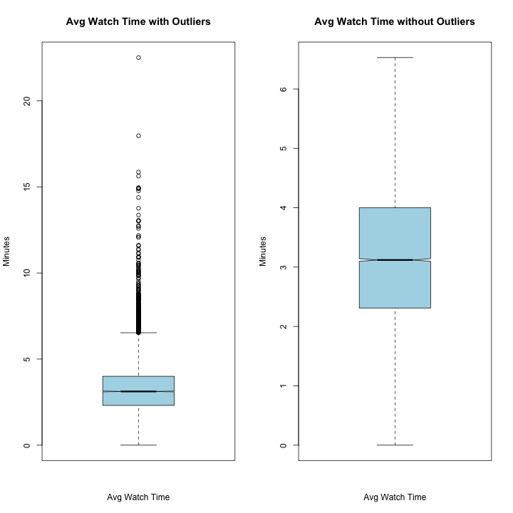
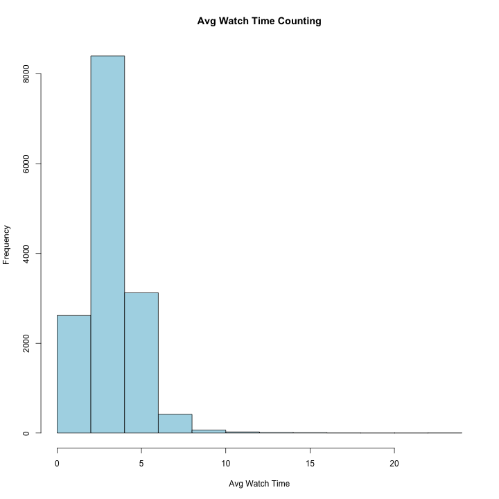
summary(rv1$average_watch_time)
##    Min. 1st Qu.  Median    Mean 3rd Qu.    Max.
##   0.000   2.310   3.120   3.232   4.000  22.510
sd(rv1$average_watch_time)
par(mfrow=c(1,2))
boxplot(rv1$average_watch_time, xlab='Avg Watch Time'
        , ylab='Minutes', main = "Avg Watch Time with Outliers",
        col="light blue", notch = TRUE, outline = TRUE)
boxplot(rv1$average_watch_time, xlab='Avg Watch Time'
        , ylab='Minutes', main = "Avg Watch Time without Outliers",
        col="light blue", notch = TRUE, outline = FALSE)
par(mfrow=c(1,1))
hist(rv1$average_watch_time, xlab='Avg Watch Time',
     main = "Avg Watch Time Counting", col="light blue")
OBSERVATION::
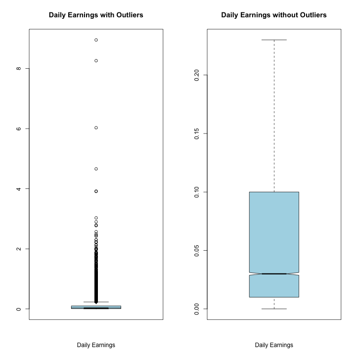
Daily Earnings Summary:
Mean: 0.1008
Standard Deviation: 0.2338
Median: 0.0300
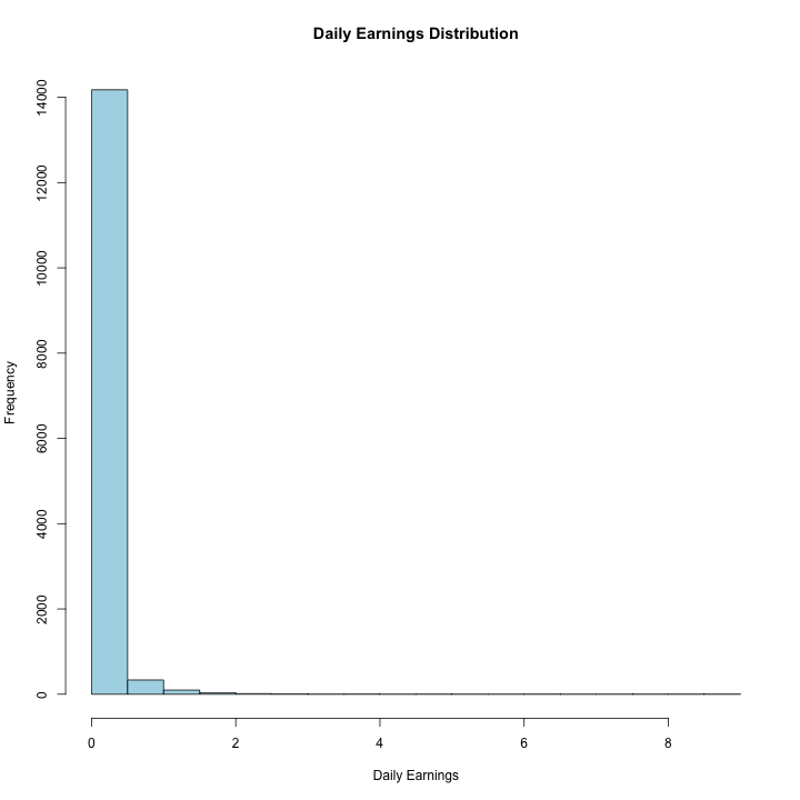
Daily Earnings shows a few significant outliers, but most of the earnings are under $1/day. The significant skew in this data indicates that most of our income can be attributed to a small number of videos. These outliers do not seem to be typos, but relevant pieces of data that tells us about the skewed nature of our profitability.
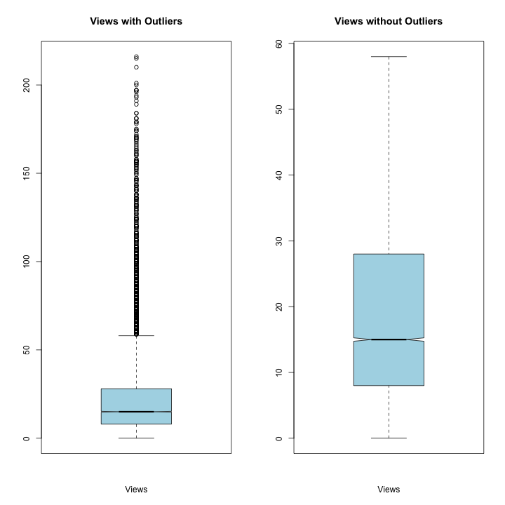
Views Summary:
Mean: 22.3
Standard Deviation: 22.97595 Median: 15.0
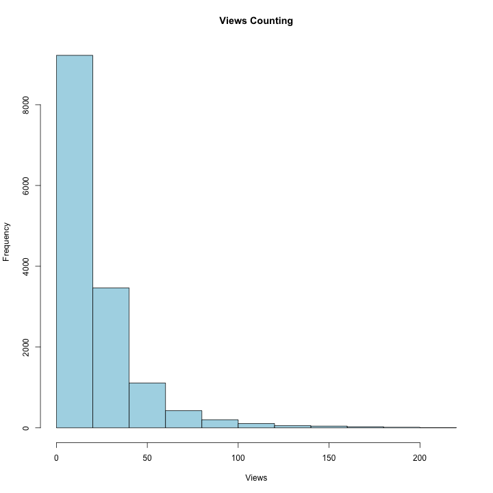
Views are also highly skewed with a long right tail. Notice the heavy right tail have significant impact on the mean as the median is smaller than the average, with the great dispersion between the number of views. Despite the indication of these outliers, we wouldn’t consider removing any data points in this case, because these are not outliers, but an indicator that a few videos are receiving a significantly larger proportion of the views.
Average Watch Time Summary:
Mean: 3.232
Standard Deviation: 1.47565 Median: 3.120
Average watch time is fairly normally distributed with a mean of 3.2 and a slight right tail. It is centered around a mean of 3.2 indicating a fairly short attention span for our viewers.
PartTwo >>>>>
Use the merged data set you constructed in Part 1 to answer the following questions:
1. During the pre-period (before Feb 5th),
i) Is average watch time different for videos that have pre-roll ads versus not? ii) Is the number of views different for videos that have pre-roll ads versus not?
For each comparison, conduct an appropriate hypothesis test, and offer an interpretation in the context of the problem.
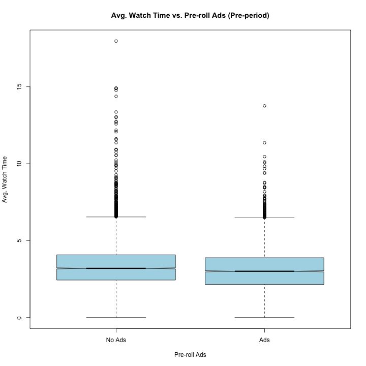
● Is the average watch time different for videos that have pre-roll ads versus not?
○ H0 = The average watch time is not different with pre-rolls ads versus those that
do not have pre-roll ads
○ H1 = The average watch time is different for videos with pre-rolls ads versus
those that do not have pre-roll ads
##Q1: During the pre-period (before Feb 5th):

#Eliminate rows with 1 in both annoy_after & before
rv2 <- rv1[-c(which(rv1$annoy_before==1 & rv1$annoy_after==1)),]  #remove inconsitancy
Q1_pre <- subset(rv2, Date < "2013-02-05" & annoy_before == "1")
Q1_no <- subset(rv2, Date < "2013-02-05" & annoy_before == "0")

#Unpaired Two-Samples T-test
t.test(Q1_pre$average_watch_time, Q1_no$average_watch_time)
##
## 	Welch Two Sample t-test
##
## data:  Q1_pre$average_watch_time and Q1_no$average_watch_time
## t = -8.3977, df = 11217, p-value < 2.2e-16
## alternative hypothesis: true difference in means is not equal to 0
## 95 percent confidence interval:
##  -0.2792857 -0.1735792
## sample estimates:
## mean of x mean of y
##  3.104515  3.330947
OBSERVATION::
This t-test tells us that we should reject the null hypothesis because the average watch time difference between videos with pre-roll ads and those without pre-roll is statistically significant. With a p-value of less than .001 and a t-test statistic of -8.3977, which translates to the mean of pre-roll average watch time being over 8 standard errors below the dataset mean of no pre-roll average watch time.
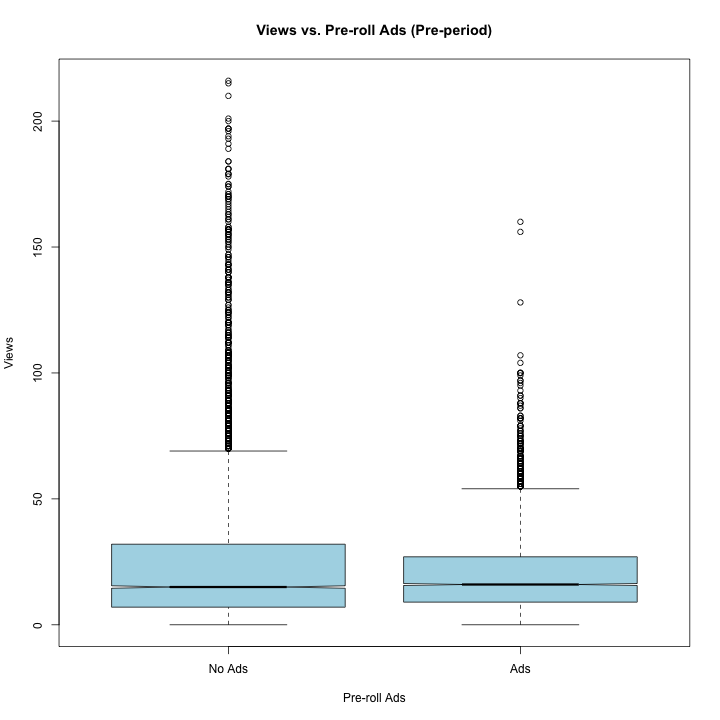
● Is the number of views different for videos that have pre-roll ads versus not?
○ H0 = The number of views is not different for videos that have pre-roll ads versus
not
○ H1 = The number of views is different for videos that have pre-roll ads versus not
t.test(Q1_pre$Views, Q1_no$Views)
##
## 	Welch Two Sample t-test
##
## data:  Q1_pre$Views and Q1_no$Views
## t = -12.159, df = 9896, p-value < 2.2e-16
## alternative hypothesis: true difference in means is not equal to 0
## 95 percent confidence interval:
##  -6.006455 -4.338688
## sample estimates:
## mean of x mean of y
##  20.12362  25.29620
OBSERVATION::
This t-test tells us that we should reject the null hypothesis because the views for videos with pre-roll ads and those without is statistically significant. With a p-value of less than .05 and a t-test statistic of -12.159, we see that the mean of pre-roll views is more than 12 standard errors below the dataset mean of no pre-roll views. Notice that with ads, views and average watch time is more spread out and significantly more right skewed.
Q1_plot <- subset(rv2, Date < "2013-02-05")
boxplot(average_watch_time~annoy_before, data=Q1_plot, col="light blue",
        main="Avg. Watch Time vs. Pre-roll Ads (Pre-period)"
        , ylab="Avg. Watch Time", xlab="Pre-roll Ads",
        names=c("No Ads","Ads"), notch = TRUE, outline = TRUE)
boxplot(Views~annoy_before, data=Q1_plot, col="light blue",
        main="Views vs. Pre-roll Ads (Pre-period)", ylab="Views", xlab="Pre-roll Ads",
        names=c("No Ads","Ads"), notch = TRUE, outline = TRUE)
2. In the full sample,
i) How does attention (measured by average watch time) relate to daily earnings on a
video? Is this relationship statistically significant?
ii) How do views relate to daily earnings on a video? Is this relationship statistically
significant?
iii) How does attention relate to views on a video? Is this relationship statistically significant?
##Q2:In the full sample:
##Relationship between daily earnings vs. average watch time?
lm_awt<- lm(rv1$daily_earnings~rv1$average_watch_time)
summary(lm_awt)
##
## Call:
## lm(formula = rv1$daily_earnings ~ rv1$average_watch_time)
##
## Residuals:
##     Min      1Q  Median      3Q     Max
## -0.1858 -0.0897 -0.0652  0.0032  8.8464
##
## Coefficients:
##                        Estimate Std. Error t value Pr(>|t|)
## (Intercept)            0.082214   0.004646  17.697  < 2e-16 ***
## rv1$average_watch_time 0.005762   0.001308   4.406 1.06e-05 ***
## ---
## Signif. codes:  0 '***' 0.001 '**' 0.01 '*' 0.05 '.' 0.1 ' ' 1
##
## Residual standard error: 0.2337 on 14667 degrees of freedom
## Multiple R-squared:  0.001322,	Adjusted R-squared:  0.001254
## F-statistic: 19.42 on 1 and 14667 DF,  p-value: 1.058e-05
par(mfrow=c(1,1))
plot(rv1$daily_earnings~rv1$average_watch_time,
     main = "Avg. Watch Time vs. Daily earnings" ,
     xlab = "Avg. Watch Time", ylab = "Daily earnings",
     lwd = 2, pch =20)
abline(coefficients(lm_awt)[1],coefficients(lm_awt)[2], col='red') #reg line

par(mfrow=c(2,2))
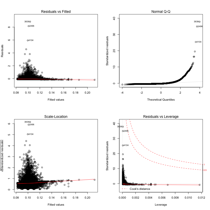
plot(lm_awt)
OBSERVATION::
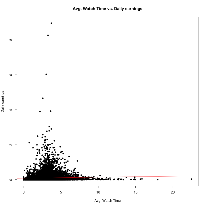
Effect of Average Watch Time on Daily Earnings: Daily_earnings = 0.082214 + 0.005762*(average_watch_time)
The relationship between these two variables is statistically significant as p-value of the slope is less than 0.05. For every one unit increase in average watch time, there is a 0.00576 dollar increase in daily earning. The intercept is statistically significant with a p-value less than 0.05. The intercept shows that at a watch time of 0 (x=0), daily earnings is predicted to be $0.0822. To us, this indicates that this intercept is meaningless or that youtubers may receive a base amount of compensation for simply uploading a video to their channel. In addition, a R-square of 0.125% indicating that 0.125% of variability in daily earnings can be explained by average watch time.
##Relationship between daily earnings vs. views?
lm_v <- lm(rv1$daily_earnings~rv1$Views)
summary(lm_v)
##
## Call:
## lm(formula = rv1$daily_earnings ~ rv1$Views)
##
## Residuals:
##     Min      1Q  Median      3Q     Max
## -0.6502 -0.0622 -0.0227  0.0165  8.5384
##
## Coefficients:
##               Estimate Std. Error t value Pr(>|t|)
## (Intercept) -3.074e-03  2.392e-03  -1.285    0.199
## rv1$Views    4.659e-03  7.471e-05  62.360   <2e-16 ***
## ---
## Signif. codes:  0 '***' 0.001 '**' 0.01 '*' 0.05 '.' 0.1 ' ' 1
##
## Residual standard error: 0.2079 on 14667 degrees of freedom
## Multiple R-squared:  0.2096,	Adjusted R-squared:  0.2095
## F-statistic:  3889 on 1 and 14667 DF,  p-value: < 2.2e-16
par(mfrow=c(1,1))
plot(rv1$daily_earnings~rv1$Views,
     main = "Views vs. Daily earnings" , xlab = "Views", ylab = "Daily earnings",
     lwd = 2, pch =20) #eliminate outliers? ylim?
abline(coefficients(lm_v)[1],coefficients(lm_v)[2], col='red') #reg line
par(mfrow=c(2,2))
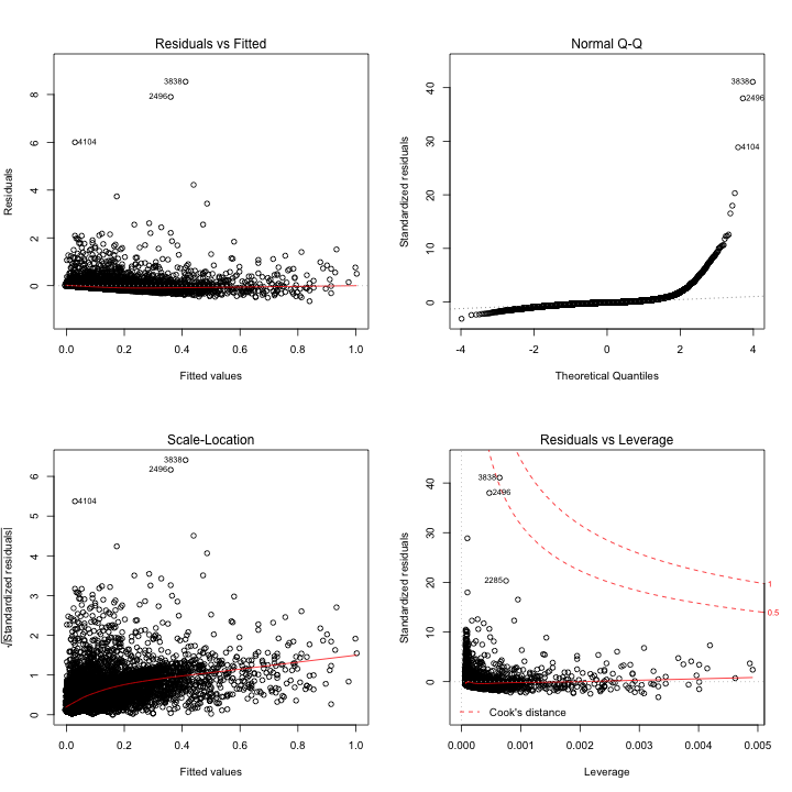
plot(lm_v)
OBSERVATION::
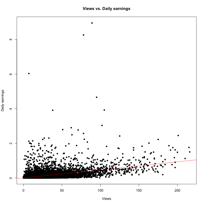
Effect of Views on Daily Earnings: Daily_earnings = -3.074e-03 + 4.659e-03*(views)
The relationship between these two variables is statistically significant because the p-value is less than 0.05. For every unit increase in views, there is a 4.659e-03 unit increase in daily earnings. The intercept is not statistically significant and is also meaningless because it impossible to have negative daily earnings (y=-3.074e-03 at x=0). In addition, a R-square of .2095 indicates that 20.95% of variability in daily earnings can be explained by views.
##Relationship between average watch time vs. views?
lm_awt_v <- lm(rv1$Views~rv1$average_watch_time)
summary(lm_awt_v)
##
## Call:
## lm(formula = rv1$Views ~ rv1$average_watch_time)
##
## Residuals:
##     Min      1Q  Median      3Q     Max
## -30.117 -14.007  -6.987   5.835 193.822
##
## Coefficients:
##                        Estimate Std. Error t value Pr(>|t|)
## (Intercept)             20.8245     0.4566  45.610  < 2e-16 ***
## rv1$average_watch_time   0.4572     0.1285   3.558 0.000375 ***
## ---
## Signif. codes:  0 '***' 0.001 '**' 0.01 '*' 0.05 '.' 0.1 ' ' 1
##
## Residual standard error: 22.97 on 14667 degrees of freedom
## Multiple R-squared:  0.0008624,	Adjusted R-squared:  0.0007942
## F-statistic: 12.66 on 1 and 14667 DF,  p-value: 0.0003749
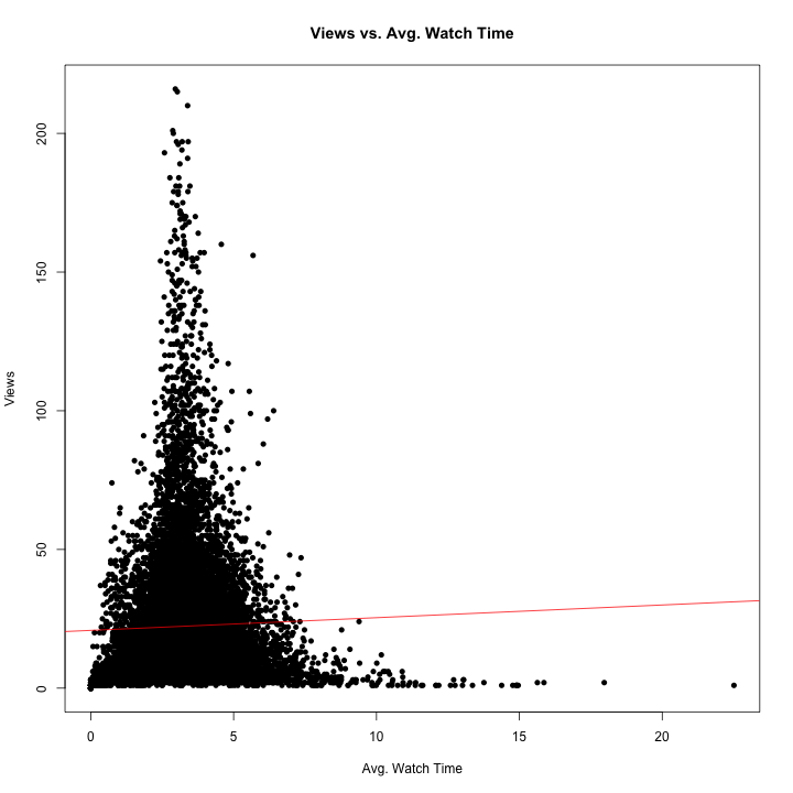
par(mfrow=c(1,1))
plot(rv1$Views~rv1$average_watch_time,
     main = "Views vs. Avg. Watch Time" , xlab = "Avg. Watch Time", ylab = "Views",
     lwd = 2, pch =20) #eliminate outliers? ylim?
abline(coefficients(lm_awt_v)[1],coefficients(lm_awt_v)[2], col='red') #reg line
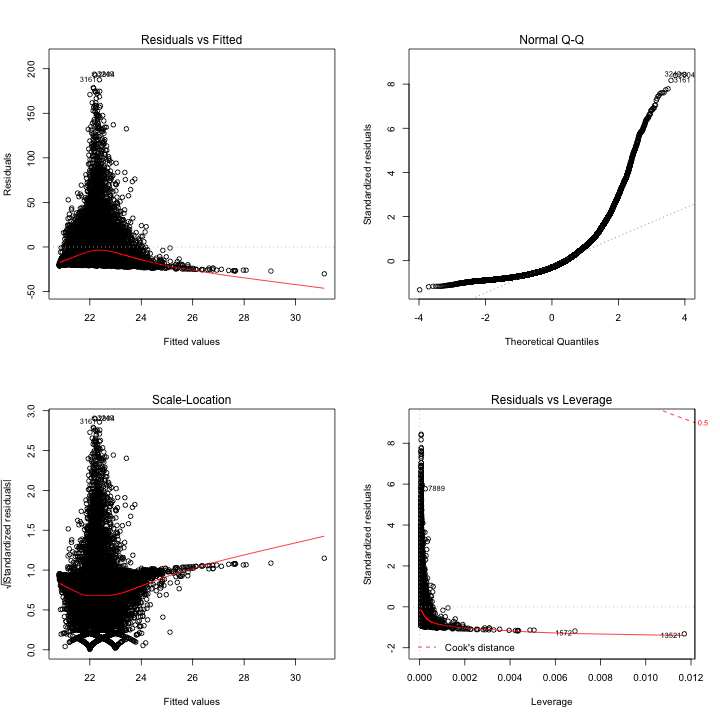
par(mfrow=c(2,2))
plot(lm_awt_v)
OBSERVATION::
Effect of Average Watch Time on Views: Views = 20.8245 + 0.4572*(average_watch_time)
The relationship between these two variables is statistically significant because the p-value is less than 0.05. For every one unit increase in average watch time, there is a 0.4572 unit increase in views. The intercept is statistically significant and meaningful with p-value less than 0.05. For an average watch time of 0 (x=0), there will be 20.82 views on average. This make sense because it is fairly common to click on a video by mistake and then quickly leave the video, registering a view but a watch time of zero. In addition, a R-square of .000794 indicates that 0.0794% of the variability in views can be explained by average watch time.
3. Define a date-level variable (named “post”) that equals whether the date is during the post period (Feb 5 or later, = 1) or during the pre period (Feb 4 or earlier, =0). Using this variable and regression tools, estimate the specification:
𝑑𝑎𝑖𝑙𝑦_𝑒𝑎𝑟𝑛𝑖𝑛𝑔𝑠,- = 𝛽0 + 𝛽2𝑝𝑜𝑠𝑡- + 𝜖,-
For your estimate of 𝛽2, is this estimate statistically significant? Interpret this estimate in the context of the problem.
##Q3:
##Relationship between post vs. daily earnings?
rv2$post <- ifelse(rv2$Date < "2013-02-05", 0, 1)
lm_p <- lm(daily_earnings~post, data=rv2)
summary(lm_p)
##
## Call:
## lm(formula = daily_earnings ~ post, data = rv2)
##
## Residuals:
##     Min      1Q  Median      3Q     Max
## -0.1042 -0.0942 -0.0642  0.0058  8.8458
##
## Coefficients:
##              Estimate Std. Error t value Pr(>|t|)
## (Intercept)  0.104190   0.002192  47.526  < 2e-16 ***
## post        -0.022166   0.004738  -4.678 2.92e-06 ***
## ---
## Signif. codes:  0 '***' 0.001 '**' 0.01 '*' 0.05 '.' 0.1 ' ' 1
##
## Residual standard error: 0.2338 on 14466 degrees of freedom
## Multiple R-squared:  0.00151,	Adjusted R-squared:  0.001441
## F-statistic: 21.88 on 1 and 14466 DF,  p-value: 2.923e-06
OBSERVATION::
Effect of Post on Daily Earnings:
Daily_earnings = 0.104190 - 0.022166*(post)
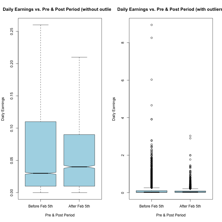
The impact of post on daily earnings is significant with a p-value less than 0.05, indicating that there is a difference in daily earnings between pre and post period. The statistically significant intercept shows that the average daily earning before February 5th is 0.104, while the average daily earnings decrease by 0.0221 after February 5th. This decrease in daily earnings can be attributed to significant outliers in daily earning before February 5th which significantly increased the overall average earnings. R-squared of .00144 indicates that 0.144% of variability in daily earnings can be explained by pre/ post-period.
In addition, the great difference in the sample size of pre (n=11371) and post period (n=3097) may have unpredictable impact the linear regression model.
par(mfrow=c(1,2))
boxplot(daily_earnings~post, data=rv2, col="light blue",
        main="Daily Earnings vs. Pre & Post Period (without outliers)", ylab="Daily Earnings", xlab="Pre & Post Period",
        names=c("Before Feb 5th","After Feb 5th"), notch = TRUE, outline = FALSE)
boxplot(daily_earnings~post, data=rv2, col="light blue",
        main="Daily Earnings vs. Pre & Post Period (with outliers)", ylab="Daily Earnings", xlab="Pre & Post Period",
        names=c("Before Feb 5th","After Feb 5th"), notch = TRUE, outline = TRUE)
4. Define a video-level variable (named “annoy_later”) that equals whether a video went from no
pre-roll advertisements to pre-roll advertisements in the post period (=1 if no pre-rollàpre-roll, =0 otherwise). Using this variable and regression tools, estimate the specification:
𝑑𝑎𝑖𝑙𝑦_𝑒𝑎𝑟𝑛𝑖𝑛𝑔𝑠,- = 𝛽0 + 𝛽2𝑎𝑛𝑛𝑜𝑦_𝑙𝑎𝑡𝑒𝑟, + 𝜖,-
For your estimate of 𝛽2, is this estimate statistically significant? Interpret this estimate in the context of the problem.
##Q4
##Relationship between annoy later vs. daily earnings?
rv2$annoy_later <- ifelse(rv2$annoy_before==0 & rv2$annoy_after==1, 1, 0)
lm_al <- lm(daily_earnings~annoy_later, data=rv2)
summary(lm_al)
##
## Call:
## lm(formula = daily_earnings ~ annoy_later, data = rv2)
##
## Residuals:
##     Min      1Q  Median      3Q     Max
## -0.1242 -0.0842 -0.0589  0.0011  8.8258
##
## Coefficients:
##             Estimate Std. Error t value Pr(>|t|)
## (Intercept) 0.068878   0.002886   23.87   <2e-16 ***
## annoy_later 0.055371   0.003884   14.26   <2e-16 ***
## ---
## Signif. codes:  0 '***' 0.001 '**' 0.01 '*' 0.05 '.' 0.1 ' ' 1
##
## Residual standard error: 0.2323 on 14466 degrees of freedom
## Multiple R-squared:  0.01385,	Adjusted R-squared:  0.01379
## F-statistic: 203.2 on 1 and 14466 DF,  p-value: < 2.2e-16
OBSERVATION::
Effect of Annoy Later on Daily Earnings:
daily earnings = 0.068878 + 0.055371*(annoy_later)
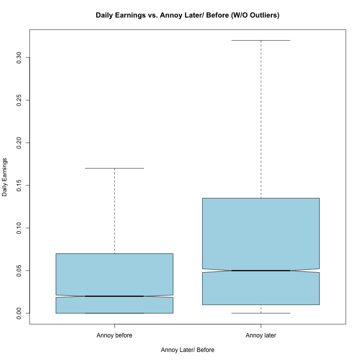
The impact of annoy_later on daily earnings was significant with a p-value of less than 0.05, indicating that there is a difference in daily earnings when videos went from no
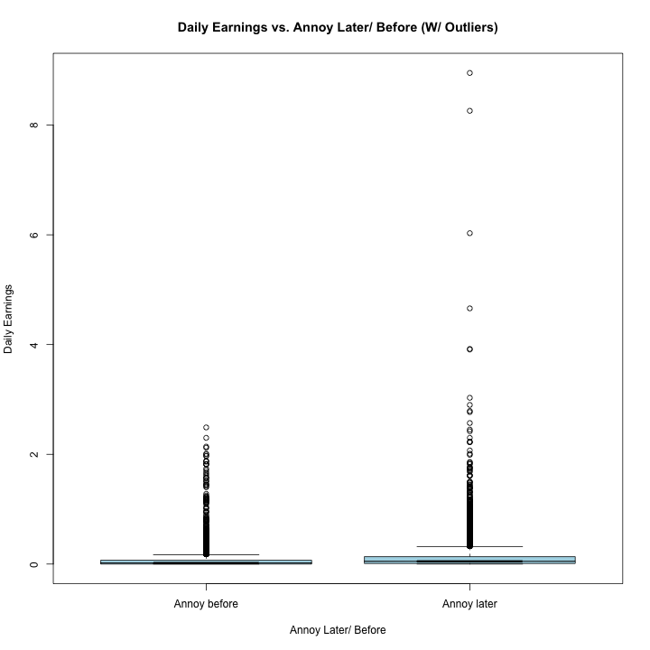
pre-roll advertisements to pre-roll advertisements and pre-roll advertisements to no pre-roll advertisements during the post period. In the other words, on average, the videos that were selected to run ads before Feb 5th are less profitable than those after Feb 5th. The statistically significant intercept shows that the average daily earning for videos chosen to pre-roll ads in pre-period is 0.0688, while the average daily earnings increase by 0.0553 for those have pre-roll ads in post-period. In addition, R-squared of 0.0137 indicates that 1.37% of variability in daily earnings can be explained by the time period of when the ads were shown (annoy later or before).
boxplot(daily_earnings~annoy_later, data=rv2, col="light blue",
        main="Daily Earnings vs. Annoy Later/ Before (W/O Outliers)"
        , ylab="Daily Earnings", xlab="Annoy Later/ Before",
        names=c("Annoy before","Annoy later"), notch = TRUE, outline = FALSE)
boxplot(daily_earnings~annoy_later, data=rv2, col="light blue",
        main="Daily Earnings vs. Annoy Later/ Before (W/ Outliers)",
        ylab="Daily Earnings", xlab="Annoy Later/ Before",
        names=c("Annoy before","Annoy later"), notch = TRUE, outline = TRUE)
5. Putting the previous two parts together, estimate the following multiple regression equation specification:
𝑑𝑎𝑖𝑙𝑦_𝑒𝑎𝑟𝑛𝑖𝑛𝑔𝑠,- = 𝛽0 + 𝛽2𝑎𝑛𝑛𝑜𝑦_𝑙𝑎𝑡𝑒𝑟, + 𝛽7𝑝𝑜𝑠𝑡- + 𝛽8𝑎𝑛𝑛𝑜𝑦_𝑙𝑎𝑡𝑒𝑟,×𝑝𝑜𝑠𝑡- + 𝜖,-
For your estimate of 𝛽8, is this estimate statistically significant? Interpret this estimate in the context of the problem.
##Q5
##Relationship between annoy later, post, and their interaction vs. daily earnings?
lm_pal <- lm(daily_earnings~post*annoy_later, data=rv2)
summary(lm_pal)
##
## Call:
## lm(formula = daily_earnings ~ post * annoy_later, data = rv2)
##
## Residuals:
##     Min      1Q  Median      3Q     Max
## -0.1343 -0.0770 -0.0570  0.0030  8.8157
##
## Coefficients:
##                   Estimate Std. Error t value Pr(>|t|)
## (Intercept)       0.066961   0.003251  20.599  < 2e-16 ***
## post              0.008918   0.007012   1.272    0.203
## annoy_later       0.067377   0.004373  15.407  < 2e-16 ***
## post:annoy_later -0.056208   0.009449  -5.949 2.76e-09 ***
## ---
## Signif. codes:  0 '***' 0.001 '**' 0.01 '*' 0.05 '.' 0.1 ' ' 1
##
## Residual standard error: 0.2319 on 14464 degrees of freedom
## Multiple R-squared:  0.01775,	Adjusted R-squared:  0.01755
## F-statistic: 87.13 on 3 and 14464 DF,  p-value: < 2.2e-16
OBSERVATION::
Effect of Post and Annoy Later (and interaction) on Daily Earnings:
Daily_Earnings = 0.066961 + 0.008918(post)+0.067377*(annoy_later)-0.056208*(post)*(annoy_later)
With the multiple regression model, the main effect of annoy later is statistically significant (p < 0.05) while the main effect of post is not. This indicates that, on average, the videos that were selected to run ads before Feb 5th make $0.0673 less than those run after Feb 5th. In previous linear regression models such as #3, the relationship shows that pre-period generates more profit than post-period, but in this model the effect of post is statistically insignificant so there is no real difference in daily earnings between videos before or after Feb 5th. However, once we combine post with annoy later, they jointly provide an explanation for daily earnings even if we do not have the statistical power to disentangle their individual effects here.
An R-squared of .0175, indicates that the two variables, annoy later and post together can explain 1.75% of the variability in daily earnings. In summary, videos without ads before Feb 5th generate highest daily earnings ($0.134), followed by videos with ads after Feb 5th ($0.0870), followed by videos with ads after Feb 5th ($0.0758) and finally without ads before Feb 5th ($0.0669).
| Daily Earnings |
Post = 0 (Before feb 5th) |
Post = 1 (After feb 5th) |
Sum across the row |
| Annoy_later = 0 (Ads during pre-period) |
0.0669 (Ads) |
0.0758 (No Ads) |
0.1427 |
| Annoy_later = 1 (Ads during post-period) |
0.134 (No Ads) |
0.0870 (Ads) |
0.221 |
| Sum across the column |
0.201 |
0.162 |
|
6. For Questions 3, 4, and 5, please repeat the analysis, but using 𝑎𝑣𝑒𝑟𝑎𝑔𝑒_𝑤𝑎𝑡𝑐h _𝑡𝑖𝑚𝑒 as the dependent variable, instead of daily earnings.
##Q6: average_watch_time and how each variable impacts it
summary(lm(average_watch_time~post, data=rv2))
##
## Call:
## lm(formula = average_watch_time ~ post, data = rv2)
##
## Residuals:
##     Min      1Q  Median      3Q     Max
## -3.3483 -0.9096 -0.1189  0.7604 19.1617
##
## Coefficients:
##             Estimate Std. Error t value Pr(>|t|)
## (Intercept)  3.22963    0.01376 234.705  < 2e-16 ***
## post         0.11862    0.02974   3.988 6.68e-05 ***
## ---
## Signif. codes:  0 '***' 0.001 '**' 0.01 '*' 0.05 '.' 0.1 ' ' 1
##
## Residual standard error: 1.467 on 14466 degrees of freedom
## Multiple R-squared:  0.001098,	Adjusted R-squared:  0.001029
## F-statistic: 15.91 on 1 and 14466 DF,  p-value: 6.682e-05
OBSERVATION::
Effect of Post on Average Watch time:
Average Watch Time = 3.22963 + 0.11862*(post)
The impact of post on average watch time was significant with a p-value less than 0.05, indicating that there is a difference in average watch time between the pre and post periods. The statistically significant intercept shows that the average watch time before February 5th is 3.22, while the average watch time increased by 0.11862 after February 5th. This might indicate that as time passed, the channel started to grab more attention. An R-squared of .00103 indicates that 0.103% of variability in average watch time can be explained by timing.
summary(lm(average_watch_time~annoy_later, data=rv2))
##
## Call:
## lm(formula = average_watch_time ~ annoy_later, data = rv2)
##
## Residuals:
##     Min      1Q  Median      3Q     Max
## -3.3416 -0.9216 -0.1216  0.7584 19.3617
##
## Coefficients:
##             Estimate Std. Error t value Pr(>|t|)
## (Intercept)  3.14827    0.01820 173.005  < 2e-16 ***
## annoy_later  0.19337    0.02449   7.895 3.11e-15 ***
## ---
## Signif. codes:  0 '***' 0.001 '**' 0.01 '*' 0.05 '.' 0.1 ' ' 1
##
## Residual standard error: 1.465 on 14466 degrees of freedom
## Multiple R-squared:  0.004291,	Adjusted R-squared:  0.004222
## F-statistic: 62.33 on 1 and 14466 DF,  p-value: 3.105e-15
OBSERVATION::
Effect of Annoy Later on Average Watch time:
average_watch_time = 3.14827 + 0.19337*(annoy_later)
The impact of annoy_later on average watch time was significant with a p-value less than 0.05, indicating that there is a difference in average watch time between videos that transitioned from no pre-roll advertisements to pre-roll advertisements and vice versa during the post period. This means that on average, the videos that were selected to run ads before Feb 5th attract more attention than those after Feb 5th. The intercept shows that the average watch time for videos chosen to run pre-roll ads in the pre-period is 3.14, while the average watch time increases by 0.193 for those that have pre-roll ads in post-period. In addition, an R-squared of .00422 indicates that 0.422% of variability in average watch time can be explained by annoy later or before.
summary(lm(average_watch_time~post*annoy_later, data=rv2))
##
## Call:
## lm(formula = average_watch_time ~ post * annoy_later, data = rv2)
##
## Residuals:
##     Min      1Q  Median      3Q     Max
## -3.3811 -0.9119 -0.1209  0.7591 19.2019
##
## Coefficients:
##                  Estimate Std. Error t value Pr(>|t|)
## (Intercept)       3.10451    0.02052 151.267  < 2e-16 ***
## post              0.20358    0.04427   4.599 4.29e-06 ***
## annoy_later       0.22643    0.02761   8.201 2.58e-16 ***
## post:annoy_later -0.15345    0.05965  -2.572   0.0101 *
## ---
## Signif. codes:  0 '***' 0.001 '**' 0.01 '*' 0.05 '.' 0.1 ' ' 1
##
## Residual standard error: 1.464 on 14464 degrees of freedom
## Multiple R-squared:  0.005852,	Adjusted R-squared:  0.005646
## F-statistic: 28.38 on 3 and 14464 DF,  p-value: < 2.2e-16
OBSERVATION::
Effect of Post and Annoy Later (and interaction) on Average Watch Time:
Average_watch_time =3.10451 +0.20358*(post) + 0.22643*(annoy_later) - 0.15345*(post)*(annoy_later)
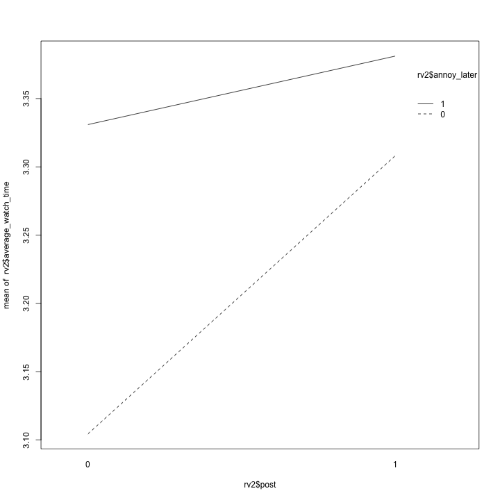
With the multiple regression model, all important variables are statistically significant (p < 0.05), including the interaction between annoy later and post. While the main effect of post and annoy later preserved the pattern observed in previous linear regression model, this model helps us identify the best and worst scenarios for achieving the highest watch time. Videos with ads after Feb 5th attracted most attention (3.381), follow by videos without ads before Feb 5th (3.33)and the videos without ads after Feb 5th (3.308), and finally, the videos with ads before Feb 5th attracted the least attention (3.104).
| Average Watch Time |
Post = 0 (Before feb 5th) |
Post = 1 (After feb 5th) |
Sum across the row |
| Annoy_later = 0 (Ads during pre-period) |
3.104 (Ads) |
3.308 (No Ads) |
6.41 |
| Annoy_later = 1 (Ads during post-period) |
3.33 (No Ads) |
3.381 (Ads) |
7.14 |
| Sum across the column |
6.43 |
6.68 |
|
interaction.plot(rv2$post, rv2$annoy_later, rv2$average_watch_time)
PartThree >>>>>
Report. Your report should provide the relevant tradeoffs for a YouTube content provider who is interested in knowing whether pre-roll advertisements will increase daily earnings, but is worried that these advertisements might reduce the amount of attention that users pay to the videos the content provider posts. If there is a significant loss of attention to the content, how much additional revenue can the content provider expect to receive to compensate for this? Please organize your discussion, graphs, and tables in a manner that is straightforward to understand for this YouTuber (who remembers loosely what a p-value is from a years-ago stats class).
#data
ads <- rbind(rv2[rv2$post==0 & rv2$annoy_later==0,]
             , rv2[rv2$post==1 & rv2$annoy_later==1,])
no_ads <- rbind(rv2[rv2$post==1 & rv2$annoy_later==0,]
                , rv2[rv2$post==0 & rv2$annoy_later==1,])

#Test to see if there is a diff in daily earnings, views, avg. watch time
t.test(ads$daily_earnings, no_ads$daily_earnings)
##
## 	Welch Two Sample t-test
##
## data:  ads$daily_earnings and no_ads$daily_earnings
## t = -13.685, df = 13366, p-value < 2.2e-16
## alternative hypothesis: true difference in means is not equal to 0
## 95 percent confidence interval:
##  -0.05913804 -0.04431981
## sample estimates:
##  mean of x  mean of y
## 0.07200088 0.12372981
t.test(ads$Views, no_ads$Views)
##
## 	Welch Two Sample t-test
##
## data:  ads$Views and no_ads$Views
## t = -8.7651, df = 13295, p-value < 2.2e-16
## alternative hypothesis: true difference in means is not equal to 0
## 95 percent confidence interval:
##  -4.005293 -2.541287
## sample estimates:
## mean of x mean of y
##  20.40297  23.67626
t.test(ads$average_watch_time, no_ads$average_watch_time)
##
## 	Welch Two Sample t-test
##
## data:  ads$average_watch_time and no_ads$average_watch_time
## t = -6.2885, df = 14432, p-value = 3.298e-10
## alternative hypothesis: true difference in means is not equal to 0
## 95 percent confidence interval:
##  -0.2005595 -0.1052409
## sample estimates:
## mean of x mean of y
##    3.1739    3.3268
###global adjustments start 2
options(warn = oldwarnval) #reset the warning message
###global adjustments end 2
CONCLUSION::
After reviewing the data, we believe we have come to several conclusions that a YouTuber can use to guide his or her decisions regarding pre-roll ads running on a channel. In general for all videos, we determined that introducing pre-roll ads when none were present decreases daily earnings, views, and average watch time (this difference is statistically significant across all variables). The magnitude of this impact varies based on other factors such as annoy later and post so more nuance can be gained from studying a particular set of users (viewers interested in economics and statistics videos may not display the same trends as those interested in popular culture). Overall, a YouTuber should think carefully about introducing ads where there were none playing before.
In general, we believe that this dataset is limited due to the following reasons: First, the videos are not popular enough to observe true differences between videos, and the statistical significance levels can be attributed more to the large sample size rather than differences in the success of videos. In addition, having low R-squared values across all analysis is concerning because it does not provide insight to where the majority of the variability is coming from for daily earnings and average watch time. There are a lot of other factors that should be explored here. Regardless of the R-square, the significant coefficients still represent the mean change in the dependent variable for one unit of change in predictor. However, notice that the R-square is so low that we won’t be able to make any precise prediction, but can predict general pattern.
Additionally, one possible confounding factor in the design of the experiment is the unequal sample size across comparison group. When analyzing the effect of the post, pre-period group contains approximately 7000 more samples than post-period, which may be a potential confounding factor.
Despite these limitations in the data, we can still use the insights from this data for help in designing future studies and making limited connections between variables that YouTubers will be interested in.
Thank you!
